Activate Client File Upload Option in Dnn Nb Store

Multivariate Time Series Forecasting with LSTMs in Keras

Last Updated on October 21, 2020

Neural networks like Long Short-Term Memory (LSTM) recurrent neural networks are able to almost seamlessly model problems with multiple input variables.

This is a great benefit in time series forecasting, where classical linear methods can be difficult to adapt to multivariate or multiple input forecasting problems.

In this tutorial, you will notice how you lot tin can develop an LSTM model for multivariate time serial forecasting with the Keras deep learning library.

After completing this tutorial, y'all volition know:

• How to transform a raw dataset into something we tin can utilise for fourth dimension series forecasting.
• How to prepare data and fit an LSTM for a multivariate fourth dimension series forecasting problem.
• How to make a forecast and rescale the event back into the original units.

Kicking-start your project with my new book Deep Learning for Time Series Forecasting, including pace-by-step tutorials and the Python source code files for all examples.

Allow's go started.

• Update Aug/2017: Fixed a bug where yhat was compared to obs at the previous time step when calculating the final RMSE. Thank you, Songbin Xu and David Righart.
• Update October/2017: Added a new example showing how to train on multiple prior time steps due to popular demand.
• Update Sep/2018: Updated link to dataset.
• Update Jun/2020: Fixed missing imports for LSTM data prep example.

Tutorial Overview

This tutorial is divided into 4 parts; they are:

1. Air Pollution Forecasting
2. Bones Information Preparation
3. Multivariate LSTM Forecast Model
   1. LSTM Data Preparation
   2. Define and Fit Model
   3. Evaluate Model
   4. Complete Example
4. Train On Multiple Lag Timesteps Example

Python Environment

This tutorial assumes you take a Python SciPy environment installed. I recommend that youuse Python iii with this tutorial.

You must have Keras (two.0 or higher) installed with either the TensorFlow or Theano backend, Ideally Keras ii.3 and TensorFlow 2.2, or higher.

The tutorial also assumes you have scikit-learn, Pandas, NumPy and Matplotlib installed.

If yous need help with your environment, see this postal service:

• How to Setup a Python Surroundings for Machine Learning

Need help with Deep Learning for Fourth dimension Series?

Take my free 7-24-hour interval email crash course now (with sample code).

Click to sign-up and too become a gratis PDF Ebook version of the course.

1. Air Pollution Forecasting

In this tutorial, we are going to employ the Air Quality dataset.

This is a dataset that reports on the conditions and the level of pollution each hour for five years at the US diplomatic mission in Beijing, Red china.

The data includes the date-time, the pollution called PM2.five concentration, and the weather information including dew point, temperature, pressure, wind direction, air current speed and the cumulative number of hours of snowfall and rain. The consummate feature list in the raw information is equally follows:

1. No: row number
2. year: year of data in this row
3. calendar month: month of information in this row
4. twenty-four hours: day of information in this row
5. 60 minutes: hour of data in this row
6. pm2.v: PM2.five concentration
7. DEWP: Dew Bespeak
8. TEMP: Temperature
9. PRES: Pressure level
10. cbwd: Combined air current management
11. Iws: Cumulated wind speed
12. Is: Cumulated hours of snow
13. Ir: Cumulated hours of rain

We can utilize this data and frame a forecasting problem where, given the weather conditions and pollution for prior hours, we forecast the pollution at the next hour.

This dataset can exist used to frame other forecasting problems.
Practice you have good ideas? Let me know in the comments below.

You tin can download the dataset from the UCI Car Learning Repository.

Update, I have mirrored the dataset here because UCI has get unreliable:

• Beijing PM2.5 Data Set

Download the dataset and place it in your electric current working directory with the filename "raw.csv".

ii. Basic Information Preparation

The data is not set to use. We must fix information technology starting time.

Below are the first few rows of the raw dataset.

No,yr,month,day,hour,pm2.5,DEWP,TEMP,PRES,cbwd,Iws,Is,Ir one,2010,i,1,0,NA,-21,-11,1021,NW,1.79,0,0 2,2010,1,ane,1,NA,-21,-12,1020,NW,4.92,0,0 3,2010,1,1,2,NA,-21,-xi,1019,NW,6.71,0,0 4,2010,1,one,iii,NA,-21,-14,1019,NW,nine.84,0,0 5,2010,i,ane,4,NA,-20,-12,1018,NW,12.97,0,0

The starting time footstep is to consolidate the date-time information into a single date-time so that we tin utilize it as an index in Pandas.

A quick check reveals NA values for pm2.5 for the start 24 hours. We will, therefore, demand to remove the outset row of data. There are too a few scattered "NA" values later in the dataset; we tin mark them with 0 values for now.

The script below loads the raw dataset and parses the date-time information equally the Pandas DataFrame alphabetize. The "No" column is dropped and and so clearer names are specified for each column. Finally, the NA values are replaced with "0" values and the get-go 24 hours are removed.

The "No" column is dropped and then clearer names are specified for each cavalcade. Finally, the NA values are replaced with "0" values and the first 24 hours are removed.

1 2 3 4 5 6 seven 8 9 10 11 12 13 fourteen 15 16 17 eighteen

from pandas import read_csv from datetime import datetime # load data def parse ( x ) : render datetime . strptime ( 10 , '%Y %m %d %H' ) dataset = read_csv ( 'raw.csv' , parse_dates = [ [ 'year' , 'month' , 'day' , 'hour' ] ] , index_col = 0 , date_parser = parse ) dataset . driblet ( 'No' , axis = 1 , inplace = True ) # manually specify column names dataset . columns = [ 'pollution' , 'dew' , 'temp' , 'press' , 'wnd_dir' , 'wnd_spd' , 'snow' , 'rain' ] dataset . index . name = 'date' # mark all NA values with 0 dataset [ 'pollution' ] . fillna ( 0 , inplace = True ) # drop the first 24 hours dataset = dataset [ 24 : ] # summarize first 5 rows print ( dataset . caput ( 5 ) ) # save to file dataset . to_csv ( 'pollution.csv' )

Running the case prints the first 5 rows of the transformed dataset and saves the dataset to "pollution.csv".

pollution  dew  temp   press wnd_dir  wnd_spd  snow  rain date 2010-01-02 00:00:00      129.0  -xvi  -four.0  1020.0      SE     1.79     0     0 2010-01-02 01:00:00      148.0  -15  -4.0  1020.0      SE     2.68     0     0 2010-01-02 02:00:00      159.0  -11  -5.0  1021.0      SE     3.57     0     0 2010-01-02 03:00:00      181.0   -7  -5.0  1022.0      SE     5.36     ane     0 2010-01-02 04:00:00      138.0   -7  -5.0  1022.0      SE     6.25     2     0

Now that we have the data in an easy-to-utilize form, we can create a quick plot of each serial and see what we have.

The code below loads the new "pollution.csv" file and plots each serial equally a separate subplot, except air current speed dir, which is chiselled.

from pandas import read_csv from matplotlib import pyplot # load dataset dataset = read_csv ( 'pollution.csv' , header = 0 , index_col = 0 ) values = dataset . values # specify columns to plot groups = [ 0 , one , 2 , 3 , 5 , 6 , 7 ] i = 1 # plot each column pyplot . figure ( ) for group in groups : pyplot . subplot ( len ( groups ) , 1 , i ) pyplot . plot ( values [ : , group ] ) pyplot . championship ( dataset . columns [ group ] , y = 0.five , loc = 'right' ) i += i pyplot . show ( )

Running the example creates a plot with 7 subplots showing the 5 years of information for each variable.

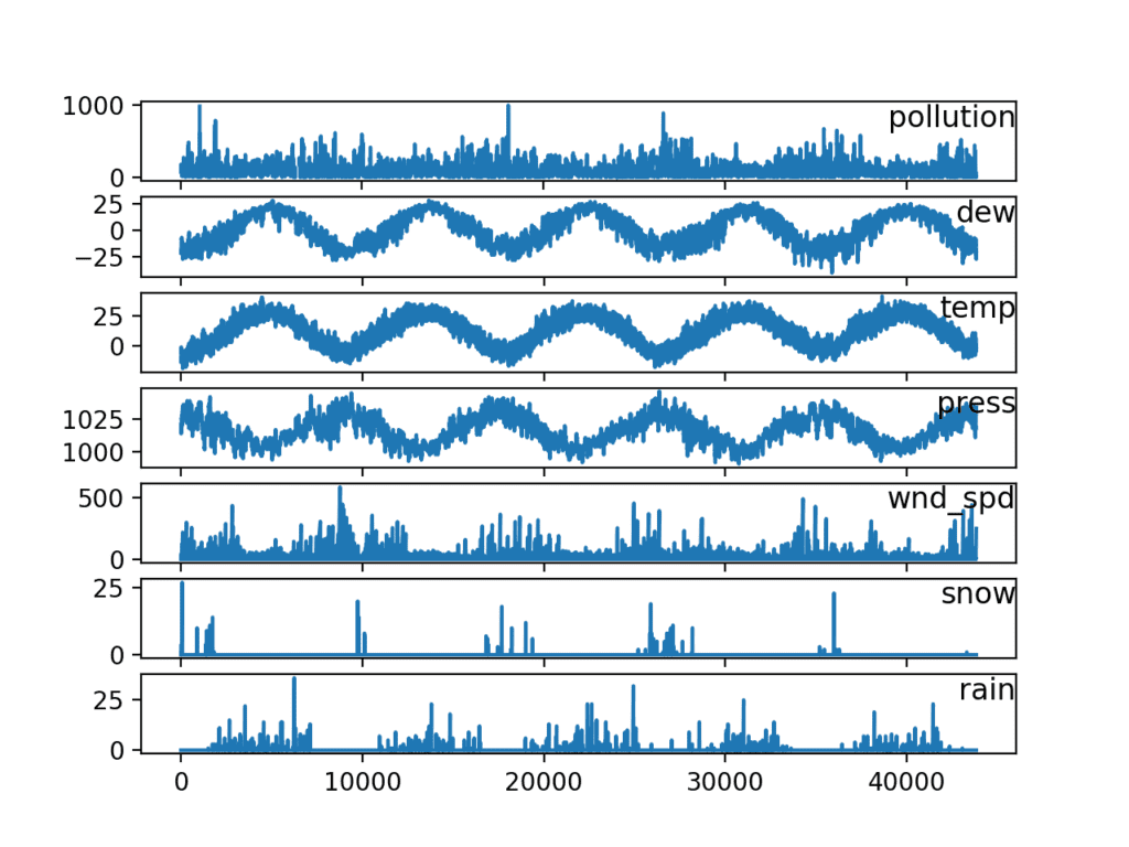
Line Plots of Air Pollution Time Series

three. Multivariate LSTM Forecast Model

In this section, we will fit an LSTM to the problem.

LSTM Data Training

The first step is to gear up the pollution dataset for the LSTM.

This involves framing the dataset as a supervised learning problem and normalizing the input variables.

We will frame the supervised learning problem as predicting the pollution at the current hr (t) given the pollution measurement and weather conditions at the prior fourth dimension step.

This formulation is straightforward and just for this demonstration. Some alternate formulations you could explore include:

• Predict the pollution for the next hour based on the weather conditions and pollution over the last 24 hours.
• Predict the pollution for the adjacent 60 minutes as higher up and given the "expected" weather atmospheric condition for the next hour.

Nosotros can transform the dataset using the series_to_supervised() function developed in the weblog postal service:

• How to Convert a Time Series to a Supervised Learning Problem in Python

First, the "pollution.csv" dataset is loaded. The wind direction feature is label encoded (integer encoded). This could further be one-hot encoded in the future if you are interested in exploring information technology.

Next, all features are normalized, then the dataset is transformed into a supervised learning problem. The weather variables for the hour to be predicted (t) are then removed.

The complete code listing is provided below.

1 ii 3 4 5 6 seven eight 9 x 11 12 thirteen 14 xv 16 17 18 xix 20 21 22 23 24 25 26 27 28 29 30 31 32 33 34 35 36 37 38 39 xl 41 42 43 44 45 46 47

# prepare data for lstm from pandas import read_csv from pandas import DataFrame from pandas import concat from sklearn . preprocessing import LabelEncoder from sklearn . preprocessing import MinMaxScaler # convert series to supervised learning def series_to_supervised ( data , n_in = 1 , n_out = 1 , dropnan = True ) : n_vars = 1 if type ( data ) is listing else data . shape [ i ] df = DataFrame ( data ) cols , names = list ( ) , listing ( ) # input sequence (t-due north, ... t-1) for i in range ( n_in , 0 , - 1 ) : cols . append ( df . shift ( i ) ) names += [ ( 'var%d(t-%d)' % ( j + 1 , i ) ) for j in range ( n_vars ) ] # forecast sequence (t, t+1, ... t+n) for i in range ( 0 , n_out ) : cols . append ( df . shift ( - i ) ) if i == 0 : names += [ ( 'var%d(t)' % ( j + ane ) ) for j in range ( n_vars ) ] else : names += [ ( 'var%d(t+%d)' % ( j + one , i ) ) for j in range ( n_vars ) ] # put information technology all together agg = concat ( cols , axis = 1 ) agg . columns = names # drop rows with NaN values if dropnan : agg . dropna ( inplace = True ) return agg # load dataset dataset = read_csv ( 'pollution.csv' , header = 0 , index_col = 0 ) values = dataset . values # integer encode direction encoder = LabelEncoder ( ) values [ : , 4 ] = encoder . fit_transform ( values [ : , 4 ] ) # ensure all data is bladder values = values . astype ( 'float32' ) # normalize features scaler = MinMaxScaler ( feature_range = ( 0 , 1 ) ) scaled = scaler . fit_transform ( values ) # frame as supervised learning reframed = series_to_supervised ( scaled , ane , 1 ) # drop columns we don't want to predict reframed . drop ( reframed . columns [ [ 9 , 10 , eleven , 12 , 13 , 14 , 15 ] ] , centrality = one , inplace = True ) print ( reframed . caput ( ) )

Running the example prints the starting time five rows of the transformed dataset. We can see the viii input variables (input serial) and the 1 output variable (pollution level at the current hour).

var1(t-ane)  var2(t-1)  var3(t-ane)  var4(t-1)  var5(t-1)  var6(t-one)  \ one   0.129779   0.352941   0.245902   0.527273   0.666667   0.002290 2   0.148893   0.367647   0.245902   0.527273   0.666667   0.003811 3   0.159960   0.426471   0.229508   0.545454   0.666667   0.005332 4   0.182093   0.485294   0.229508   0.563637   0.666667   0.008391 5   0.138833   0.485294   0.229508   0.563637   0.666667   0.009912    var7(t-1)  var8(t-1)   var1(t) 1   0.000000        0.0  0.148893 2   0.000000        0.0  0.159960 3   0.000000        0.0  0.182093 four   0.037037        0.0  0.138833 5   0.074074        0.0  0.109658

This data preparation is simple and there is more than nosotros could explore. Some ideas yous could look at include:

• One-hot encoding wind management.
• Making all series stationary with differencing and seasonal adjustment.
• Providing more than 1 hour of input time steps.

This final indicate is mayhap the most important given the use of Backpropagation through time past LSTMs when learning sequence prediction problems.

Define and Fit Model

In this section, nosotros will fit an LSTM on the multivariate input data.

First, we must split the prepared dataset into railroad train and exam sets. To speed upward the training of the model for this demonstration, we will only fit the model on the starting time year of information, then evaluate information technology on the remaining 4 years of data. If you have time, consider exploring the inverted version of this exam harness.

The example below splits the dataset into railroad train and examination sets, then splits the train and test sets into input and output variables. Finally, the inputs (Ten) are reshaped into the 3D format expected by LSTMs, namely [samples, timesteps, features].

. . . # split into train and test sets values = reframed . values n_train_hours = 365 * 24 railroad train = values [ : n_train_hours , : ] test = values [ n_train_hours : , : ] # split into input and outputs train_X , train_y = train [ : , : - 1 ] , train [ : , - 1 ] test_X , test_y = test [ : , : - i ] , test [ : , - 1 ] # reshape input to be 3D [samples, timesteps, features] train_X = train_X . reshape ( ( train_X . shape [ 0 ] , one , train_X . shape [ ane ] ) ) test_X = test_X . reshape ( ( test_X . shape [ 0 ] , i , test_X . shape [ 1 ] ) ) print ( train_X . shape , train_y . shape , test_X . shape , test_y . shape )

Running this case prints the shape of the train and test input and output sets with most 9K hours of data for training and near 35K hours for testing.

(8760, i, 8) (8760,) (35039, 1, 8) (35039,)

At present nosotros can define and fit our LSTM model.

We will define the LSTM with 50 neurons in the first hidden layer and 1 neuron in the output layer for predicting pollution. The input shape volition be 1 time step with viii features.

Nosotros volition employ the Hateful Absolute Error (MAE) loss function and the efficient Adam version of stochastic slope descent.

The model volition exist fit for 50 training epochs with a batch size of 72. Remember that the internal land of the LSTM in Keras is reset at the terminate of each batch, and then an internal state that is a part of a number of days may be helpful (attempt testing this).

Finally, we continue rails of both the training and examination loss during training by setting the validation_data statement in the fit() function. At the end of the run both the training and test loss are plotted.

. . . # design network model = Sequential ( ) model . add together ( LSTM ( 50 , input_shape = ( train_X . shape [ i ] , train_X . shape [ 2 ] ) ) ) model . add ( Dense ( 1 ) ) model . compile ( loss = 'mae' , optimizer = 'adam' ) # fit network history = model . fit ( train_X , train_y , epochs = 50 , batch_size = 72 , validation_data = ( test_X , test_y ) , verbose = 2 , shuffle = False ) # plot history pyplot . plot ( history . history [ 'loss' ] , characterization = 'train' ) pyplot . plot ( history . history [ 'val_loss' ] , label = 'test' ) pyplot . legend ( ) pyplot . show ( )

Evaluate Model

Subsequently the model is fit, nosotros can forecast for the unabridged test dataset.

We combine the forecast with the test dataset and invert the scaling. We also invert scaling on the test dataset with the expected pollution numbers.

With forecasts and actual values in their original calibration, we can then calculate an fault score for the model. In this case, nosotros calculate the Root Mean Squared Error (RMSE) that gives error in the same units as the variable itself.

. . . # make a prediction yhat = model . predict ( test_X ) test_X = test_X . reshape ( ( test_X . shape [ 0 ] , test_X . shape [ two ] ) ) # invert scaling for forecast inv_yhat = concatenate ( ( yhat , test_X [ : , one : ] ) , centrality = 1 ) inv_yhat = scaler . inverse_transform ( inv_yhat ) inv_yhat = inv_yhat [ : , 0 ] # invert scaling for bodily test_y = test_y . reshape ( ( len ( test_y ) , 1 ) ) inv_y = concatenate ( ( test_y , test_X [ : , one : ] ) , axis = 1 ) inv_y = scaler . inverse_transform ( inv_y ) inv_y = inv_y [ : , 0 ] # calculate RMSE rmse = sqrt ( mean_squared_error ( inv_y , inv_yhat ) ) print ( 'Examination RMSE: %.3f' % rmse )

Consummate Case

The complete instance is listed beneath.

NOTE: This example assumes y'all have prepared the data correctly, eastward.thousand. converted the downloaded "raw.csv" to the prepared "pollution.csv". See the first part of this tutorial.

1 2 3 four five 6 7 8 9 ten eleven 12 13 14 15 sixteen 17 18 xix 20 21 22 23 24 25 26 27 28 29 thirty 31 32 33 34 35 36 37 38 39 forty 41 42 43 44 45 46 47 48 49 l 51 52 53 54 55 56 57 58 59 60 61 62 63 64 65 66 67 68 69 70 71 72 73 74 75 76 77 78 79 80 81 82 83 84 85 86 87 88 89 ninety 91 92 93 94 95

from math import sqrt from numpy import concatenate from matplotlib import pyplot from pandas import read_csv from pandas import DataFrame from pandas import concat from sklearn . preprocessing import MinMaxScaler from sklearn . preprocessing import LabelEncoder from sklearn . metrics import mean_squared_error from keras . models import Sequential from keras . layers import Dense from keras . layers import LSTM # convert serial to supervised learning def series_to_supervised ( information , n_in = 1 , n_out = 1 , dropnan = True ) : n_vars = i if type ( data ) is list else data . shape [ 1 ] df = DataFrame ( data ) cols , names = list ( ) , listing ( ) # input sequence (t-n, ... t-ane) for i in range ( n_in , 0 , - i ) : cols . append ( df . shift ( i ) ) names += [ ( 'var%d(t-%d)' % ( j + 1 , i ) ) for j in range ( n_vars ) ] # forecast sequence (t, t+1, ... t+n) for i in range ( 0 , n_out ) : cols . suspend ( df . shift ( - i ) ) if i == 0 : names += [ ( 'var%d(t)' % ( j + 1 ) ) for j in range ( n_vars ) ] else : names += [ ( 'var%d(t+%d)' % ( j + 1 , i ) ) for j in range ( n_vars ) ] # put it all together agg = concat ( cols , axis = ane ) agg . columns = names # drop rows with NaN values if dropnan : agg . dropna ( inplace = True ) render agg # load dataset dataset = read_csv ( 'pollution.csv' , header = 0 , index_col = 0 ) values = dataset . values # integer encode direction encoder = LabelEncoder ( ) values [ : , 4 ] = encoder . fit_transform ( values [ : , 4 ] ) # ensure all data is float values = values . astype ( 'float32' ) # normalize features scaler = MinMaxScaler ( feature_range = ( 0 , 1 ) ) scaled = scaler . fit_transform ( values ) # frame equally supervised learning reframed = series_to_supervised ( scaled , 1 , 1 ) # drop columns nosotros don't desire to predict reframed . drop ( reframed . columns [ [ 9 , ten , eleven , 12 , 13 , 14 , 15 ] ] , axis = 1 , inplace = True ) print ( reframed . head ( ) ) # split into train and test sets values = reframed . values n_train_hours = 365 * 24 train = values [ : n_train_hours , : ] test = values [ n_train_hours : , : ] # split into input and outputs train_X , train_y = train [ : , : - 1 ] , train [ : , - 1 ] test_X , test_y = examination [ : , : - 1 ] , test [ : , - 1 ] # reshape input to exist 3D [samples, timesteps, features] train_X = train_X . reshape ( ( train_X . shape [ 0 ] , 1 , train_X . shape [ 1 ] ) ) test_X = test_X . reshape ( ( test_X . shape [ 0 ] , 1 , test_X . shape [ one ] ) ) print ( train_X . shape , train_y . shape , test_X . shape , test_y . shape ) # design network model = Sequential ( ) model . add ( LSTM ( fifty , input_shape = ( train_X . shape [ 1 ] , train_X . shape [ 2 ] ) ) ) model . add ( Dense ( ane ) ) model . compile ( loss = 'mae' , optimizer = 'adam' ) # fit network history = model . fit ( train_X , train_y , epochs = 50 , batch_size = 72 , validation_data = ( test_X , test_y ) , verbose = ii , shuffle = False ) # plot history pyplot . plot ( history . history [ 'loss' ] , label = 'train' ) pyplot . plot ( history . history [ 'val_loss' ] , label = 'test' ) pyplot . legend ( ) pyplot . show ( ) # brand a prediction yhat = model . predict ( test_X ) test_X = test_X . reshape ( ( test_X . shape [ 0 ] , test_X . shape [ two ] ) ) # invert scaling for forecast inv_yhat = concatenate ( ( yhat , test_X [ : , 1 : ] ) , centrality = 1 ) inv_yhat = scaler . inverse_transform ( inv_yhat ) inv_yhat = inv_yhat [ : , 0 ] # invert scaling for actual test_y = test_y . reshape ( ( len ( test_y ) , 1 ) ) inv_y = concatenate ( ( test_y , test_X [ : , 1 : ] ) , axis = 1 ) inv_y = scaler . inverse_transform ( inv_y ) inv_y = inv_y [ : , 0 ] # calculate RMSE rmse = sqrt ( mean_squared_error ( inv_y , inv_yhat ) ) print ( 'Test RMSE: %.3f' % rmse )

Running the example first creates a plot showing the train and examination loss during grooming.

Annotation: Your results may vary given the stochastic nature of the algorithm or evaluation process, or differences in numerical precision. Consider running the example a few times and compare the boilerplate outcome.

Interestingly, we tin can see that test loss drops beneath training loss. The model may be overfitting the training information. Measuring and plotting RMSE during training may shed more light on this.

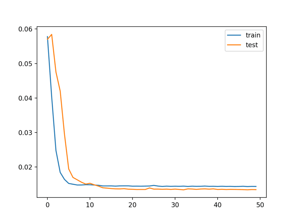
Line Plot of Train and Test Loss from the Multivariate LSTM During Training

The Train and test loss are printed at the end of each preparation epoch. At the end of the run, the final RMSE of the model on the test dataset is printed.

We can run into that the model achieves a respectable RMSE of 26.496, which is lower than an RMSE of 30 establish with a persistence model.

... Epoch 46/50 0s - loss: 0.0143 - val_loss: 0.0133 Epoch 47/50 0s - loss: 0.0143 - val_loss: 0.0133 Epoch 48/fifty 0s - loss: 0.0144 - val_loss: 0.0133 Epoch 49/fifty 0s - loss: 0.0143 - val_loss: 0.0133 Epoch 50/50 0s - loss: 0.0144 - val_loss: 0.0133 Examination RMSE: 26.496

This model is not tuned. Can you do better?
Let me know your trouble framing, model configuration, and RMSE in the comments below.

Train On Multiple Lag Timesteps Example

There take been many requests for advice on how to adapt the above example to railroad train the model on multiple previous fourth dimension steps.

I had tried this and a myriad of other configurations when writing the original post and decided non to include them considering they did not lift model skill.

Nevertheless, I have included this example beneath as reference template that you could adapt for your own issues.

The changes needed to train the model on multiple previous fourth dimension steps are quite minimal, as follows:

First, yous must frame the problem suitably when calling series_to_supervised(). We will apply three hours of data equally input. Also note, nosotros no longer explictly drib the columns from all of the other fields at ob(t).

. . . # specify the number of lag hours n_hours = 3 n_features = 8 # frame as supervised learning reframed = series_to_supervised ( scaled , n_hours , one )

Adjacent, we demand to be more conscientious in specifying the cavalcade for input and output.

We have three * 8 + 8 columns in our framed dataset. We will take 3 * 8 or 24 columns as input for the obs of all features across the previous three hours. We volition take just the pollution variable as output at the following hr, as follows:

. . . # split into input and outputs n_obs = n_hours * n_features train_X , train_y = train [ : , : n_obs ] , railroad train [ : , - n_features ] test_X , test_y = test [ : , : n_obs ] , test [ : , - n_features ] impress ( train_X . shape , len ( train_X ) , train_y . shape )

Adjacent, we tin reshape our input data correctly to reverberate the fourth dimension steps and features.

. . . # reshape input to exist 3D [samples, timesteps, features] train_X = train_X . reshape ( ( train_X . shape [ 0 ] , n_hours , n_features ) ) test_X = test_X . reshape ( ( test_X . shape [ 0 ] , n_hours , n_features ) )

Fitting the model is the aforementioned.

The just other pocket-sized change is in how to evaluate the model. Specifically, in how we reconstruct the rows with 8 columns suitable for reversing the scaling performance to get the y and yhat back into the original calibration so that we tin can calculate the RMSE.

The gist of the change is that we concatenate the y or yhat column with the last vii features of the examination dataset in order to inverse the scaling, as follows:

. . . # invert scaling for forecast inv_yhat = concatenate ( ( yhat , test_X [ : , - 7 : ] ) , axis = 1 ) inv_yhat = scaler . inverse_transform ( inv_yhat ) inv_yhat = inv_yhat [ : , 0 ] # invert scaling for actual test_y = test_y . reshape ( ( len ( test_y ) , i ) ) inv_y = concatenate ( ( test_y , test_X [ : , - 7 : ] ) , centrality = 1 ) inv_y = scaler . inverse_transform ( inv_y ) inv_y = inv_y [ : , 0 ]

We can tie all of these modifications to the above case together. The complete example of multvariate fourth dimension series forecasting with multiple lag inputs is listed below:

1 2 3 4 v 6 7 eight 9 x 11 12 thirteen fourteen 15 sixteen 17 xviii 19 20 21 22 23 24 25 26 27 28 29 30 31 32 33 34 35 36 37 38 39 40 41 42 43 44 45 46 47 48 49 50 51 52 53 54 55 56 57 58 59 60 61 62 63 64 65 66 67 68 69 70 71 72 73 74 75 76 77 78 79 80 81 82 83 84 85 86 87 88 89 90 91 92 93 94 95 96 97 98

from math import sqrt from numpy import concatenate from matplotlib import pyplot from pandas import read_csv from pandas import DataFrame from pandas import concat from sklearn . preprocessing import MinMaxScaler from sklearn . preprocessing import LabelEncoder from sklearn . metrics import mean_squared_error from keras . models import Sequential from keras . layers import Dumbo from keras . layers import LSTM # convert series to supervised learning def series_to_supervised ( information , n_in = i , n_out = 1 , dropnan = Truthful ) : n_vars = 1 if blazon ( data ) is list else data . shape [ i ] df = DataFrame ( data ) cols , names = list ( ) , list ( ) # input sequence (t-northward, ... t-1) for i in range ( n_in , 0 , - 1 ) : cols . append ( df . shift ( i ) ) names += [ ( 'var%d(t-%d)' % ( j + 1 , i ) ) for j in range ( n_vars ) ] # forecast sequence (t, t+1, ... t+due north) for i in range ( 0 , n_out ) : cols . append ( df . shift ( - i ) ) if i == 0 : names += [ ( 'var%d(t)' % ( j + i ) ) for j in range ( n_vars ) ] else : names += [ ( 'var%d(t+%d)' % ( j + i , i ) ) for j in range ( n_vars ) ] # put information technology all together agg = concat ( cols , axis = one ) agg . columns = names # drib rows with NaN values if dropnan : agg . dropna ( inplace = True ) return agg # load dataset dataset = read_csv ( 'pollution.csv' , header = 0 , index_col = 0 ) values = dataset . values # integer encode direction encoder = LabelEncoder ( ) values [ : , four ] = encoder . fit_transform ( values [ : , 4 ] ) # ensure all data is float values = values . astype ( 'float32' ) # normalize features scaler = MinMaxScaler ( feature_range = ( 0 , i ) ) scaled = scaler . fit_transform ( values ) # specify the number of lag hours n_hours = 3 n_features = 8 # frame as supervised learning reframed = series_to_supervised ( scaled , n_hours , i ) impress ( reframed . shape ) # divide into railroad train and exam sets values = reframed . values n_train_hours = 365 * 24 train = values [ : n_train_hours , : ] test = values [ n_train_hours : , : ] # split up into input and outputs n_obs = n_hours * n_features train_X , train_y = train [ : , : n_obs ] , train [ : , - n_features ] test_X , test_y = exam [ : , : n_obs ] , test [ : , - n_features ] print ( train_X . shape , len ( train_X ) , train_y . shape ) # reshape input to be 3D [samples, timesteps, features] train_X = train_X . reshape ( ( train_X . shape [ 0 ] , n_hours , n_features ) ) test_X = test_X . reshape ( ( test_X . shape [ 0 ] , n_hours , n_features ) ) print ( train_X . shape , train_y . shape , test_X . shape , test_y . shape ) # design network model = Sequential ( ) model . add ( LSTM ( l , input_shape = ( train_X . shape [ 1 ] , train_X . shape [ 2 ] ) ) ) model . add ( Dense ( ane ) ) model . compile ( loss = 'mae' , optimizer = 'adam' ) # fit network history = model . fit ( train_X , train_y , epochs = fifty , batch_size = 72 , validation_data = ( test_X , test_y ) , verbose = 2 , shuffle = False ) # plot history pyplot . plot ( history . history [ 'loss' ] , characterization = 'train' ) pyplot . plot ( history . history [ 'val_loss' ] , label = 'exam' ) pyplot . legend ( ) pyplot . evidence ( ) # make a prediction yhat = model . predict ( test_X ) test_X = test_X . reshape ( ( test_X . shape [ 0 ] , n_hours* n_features ) ) # capsize scaling for forecast inv_yhat = concatenate ( ( yhat , test_X [ : , - 7 : ] ) , axis = 1 ) inv_yhat = scaler . inverse_transform ( inv_yhat ) inv_yhat = inv_yhat [ : , 0 ] # capsize scaling for actual test_y = test_y . reshape ( ( len ( test_y ) , ane ) ) inv_y = concatenate ( ( test_y , test_X [ : , - 7 : ] ) , centrality = 1 ) inv_y = scaler . inverse_transform ( inv_y ) inv_y = inv_y [ : , 0 ] # summate RMSE rmse = sqrt ( mean_squared_error ( inv_y , inv_yhat ) ) print ( 'Test RMSE: %.3f' % rmse )

Note: Your results may vary given the stochastic nature of the algorithm or evaluation process, or differences in numerical precision. Consider running the instance a few times and compare the average event.

The model is fit as before in a minute or 2.

... Epoch 45/50 1s - loss: 0.0143 - val_loss: 0.0154 Epoch 46/fifty 1s - loss: 0.0143 - val_loss: 0.0148 Epoch 47/fifty 1s - loss: 0.0143 - val_loss: 0.0152 Epoch 48/50 1s - loss: 0.0143 - val_loss: 0.0151 Epoch 49/50 1s - loss: 0.0143 - val_loss: 0.0152 Epoch 50/50 1s - loss: 0.0144 - val_loss: 0.0149

A plot of train and test loss over the epochs is plotted.

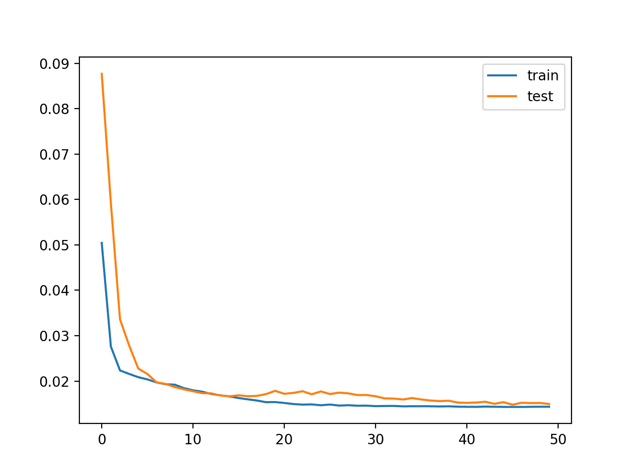
Plot of Loss on the Train and Examination Datasets

Finally, the Test RMSE is printed, not really showing any advantage in skill, at least on this problem.

I would add that the LSTM does not appear to be suitable for autoregression type problems and that you may be amend off exploring an MLP with a large window.

I hope this example helps you with your own time series forecasting experiments.

Further Reading

This department provides more resources on the topic if yous are looking go deeper.

• Beijing PM2.5 Information Set on the UCI Automobile Learning Repository
• The 5 Step Life-Cycle for Long Curt-Term Memory Models in Keras
• Time Series Forecasting with the Long Brusque-Term Retentivity Network in Python
• Multi-pace Fourth dimension Series Forecasting with Long Short-Term Memory Networks in Python

Summary

In this tutorial, you discovered how to fit an LSTM to a multivariate fourth dimension series forecasting trouble.

Specifically, you learned:

• How to transform a raw dataset into something we can utilize for time series forecasting.
• How to gear up data and fit an LSTM for a multivariate fourth dimension series forecasting problem.
• How to make a forecast and rescale the result back into the original units.

Do you accept whatsoever questions?
Ask your questions in the comments below and I volition do my best to answer.

Develop Deep Learning models for Fourth dimension Serial Today!

Develop Your Ain Forecasting models in Minutes

...with but a few lines of python code

Discover how in my new Ebook:
Deep Learning for Fourth dimension Serial Forecasting

Information technology provides self-report tutorials on topics like:
CNNs, LSTMs, Multivariate Forecasting, Multi-Stride Forecasting and much more...

Finally Bring Deep Learning to your Time Series Forecasting Projects

Skip the Academics. Just Results.

Run across What'due south Inside

kulikowskidins1974.blogspot.com

Source: https://machinelearningmastery.com/multivariate-time-series-forecasting-lstms-keras/

Share this post